Data structure
R is an object-oriented language: an object in R is anything (constants, data structures, functions, graphs) that can be assigned to a variable:
Data Objects: used to store real or complex numerical values, logical values or characters. These objects are always vectors: there are no scalars in R.
Language Objects: functions, expressions
Data structure types
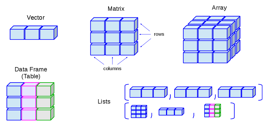
Vectors: one-dimensional arrays used to store collection data of the same mode
Numeric Vectors (mode: numeric)
Complex Vectors (mode: complex)
Logical Vectors (model: logical)
Character Vector or text strings (mode: character)
Matrices: two-dimensional arrays to store collections of data of the same mode. They are accessed by two integer indices.
Arrays: similar to matrices but they can be multi-dimensional (more than two dimensions)
Factors: vectors of categorical variables designed to group the components of another vector with the same size
Lists: ordered collection of objects, where the elements can be of different types
Data Frames: generalization of matrices where different columns can store different mode data.
Functions: objects created by the user and reused to make specific operations.
Vectors
Numeric Vectors
There are several ways to assign values to a variable:
> a <- 1.7               # assign a value to a vector with only one element (~ scalar)
> 1.7 -> a              # assign a value to a vector with only one element (~ scalar)
> a = 1.7                # assign a value to a vector with only one element (~ scalar)
> assign("a", 1.7)      # assign a value to a vector with only one element (~ scalar)
To show the values:
> a                     # show the value in the screen (not valid in scripts)
[1] 1.7
> print(a)              # show the value in the screen (valid in scripts)
[1] 1.7
Scalars (i.e., individual numbers), do not really exist in R. What appear to be individual numbers are actually one-element vectors:
> a[1]
[1] 1.7
To generate a vector with several numeric values:
> a <- c(10, 11, 15, 19) # assign four values to a vector using the concatenate command c()
> a                      # show the value in the screen
[1] 10 11 15 19
The operations are always done over all the elements of the numeric array:
> a*a                   # evaluate the square value of every element in the vector
[1] 100 121 225 361
> 1/a                   # evaluate the inverse value of every element in the vector
[1] 0.10000000 0.09090909 0.06666667 0.05263158
> b <- a-1              # subtract 1 from every element and assign the result to b
> b
[1]  9 10 14 18
To generate a sequence:
> 2:10                               # generate a sequence from n1=2 to n2=10 using n1:n2
[1]  2  3  4  5  6  7  8  9 10
> 5:1                                # generate an inverse sequence if n2 < n1
[1] 5 4 3 2 1

> seq(from=n1, to=n2, by=n3)         # generate sequence from n1 to n2 using n3 step
                                     #  (parameters names can be avoided if order is kept)
> seq(from=1, to=10, by=3)
[1]  1  4  7 10
> seq(1, 10, 3)
[1]  1  4  7 10

> seq(length=10, from=1, by=3)       # generate a fixed length sequence
[1]  1  4  7 10 13 16 19 22 25 28

> help(seq)                          # for help about this command
...
To generate repetitions:
> a <- 1:3; b <- rep(a, times=3); c <- rep(a, each=3) # command rep()
In the previous example we have run three commands in the same line. They have
been separated by a ;.
The content of the three variables is now:
> a
[1] 1 2 3
> b
[1] 1 2 3 1 2 3 1 2 3
> c
[1] 1 1 1 2 2 2 3 3 3
The recycling rule: vectors of different sizes can be combined, as far as the length of the longer vector is a multiple of the shorter vector’s length (otherwise a warning is issued, although the operation is carried out):
> a + c                                       # proper dimensions
[1] 2 3 4 3 4 5 4 5 6                         # (operation equivalent to b+c)
> d <- c(10,100)
> b + d                                       # incorrect dimensions
[1]  11 102  13 101  12 103  11 102  13
Warning message:
In b + d : longer object length is not a multiple of shorter object length
If we need to know which are the objects that are currently defined, we can list them:
> ls()
[1] "a" "b" "c" "d"
Undesired objects can be deleted using rm() function:
> rm(a, c)                                   # remove objects 'a' and 'b'
> ls()                                       # list current objects
[1] "b" "d"
In order to remove everything in the working environment:
> rm(list=ls())                               # Use this with caution
> ls()                                        # (you'll receive no warning!)
character(0)
Logical Vectors
> a <- seq(1:10)                             # generate a sequence
> a
[1]  1  2  3  4  5  6  7  8  9 10             # show values in screen
> b <- (a>5)                                 # assign values from an inequality
> b                                          # show values in screen
[1] FALSE FALSE FALSE FALSE FALSE  TRUE  TRUE  TRUE  TRUE  TRUE
> a[b]                                       # show values that fulfil the condition
[1]  6  7  8  9 10
> a[a>5]                                     # the same, but avoiding intermediate variable
[1]  6  7  8  9 10
Character Vectors
> a <- "This is an example"                  # generate a character vector
> a                                          # show vector content
[1] "This is an example"
We can concatenate vectors after converting them into character vectors:
> x <- 1.5
> y <- -2.7
> paste("Point is (",x,",",y,")", sep="")    # concatenate x, y and a string using 'paste'
[1] "Point is (1.5,-2.7)"
Matrices
A matrix is a bi-dimensional collection of data:
> a <- matrix(1:12, nrow=3, ncol=4)          # define a matrix with 3 rows and 4 columns
> a
   [,1] [,2] [,3] [,4]
[1,]    1    4    7   10
[2,]    2    5    8   11
[3,]    3    6    9   12

> dim(a)                                     # return matrix dimensions (rows,columns)
[1] 3 4
The elements of vectors and matrices are recycled when it is required by the involved dimensions:
> a <- matrix(1:8, nrow=4, ncol=4)           # create a matrix with 4 rows and 4 columns
> a
     [,1] [,2] [,3] [,4]
[1,]    1    5    1    5
[2,]    2    6    2    6
[3,]    3    7    3    7
[4,]    4    8    4    8
Arrays
They are similar to the matrices although they can have 2 o more dimensions.
> z <- array(1:24, dim=c(2,3,4))
> z
, , 1

      [,1] [,2] [,3]
[1,]    1    3    5
[2,]    2    4    6

, , 2

      [,1] [,2] [,3]
[1,]    7    9   11
[2,]    8   10   12

, , 3

      [,1] [,2] [,3]
[1,]   13   15   17
[2,]   14   16   18

, , 4

      [,1] [,2] [,3]
[1,]   19   21   23
[2,]   20   22   24
Factors
Factors are vectors that contain categorical information useful to group the values of other vectors of the same size. Let’s see an example:
# (B-V) colours from 13 galaxies
> bv <- c(0.92,0.97,0.87,0.91,0.92,1.04,0.91,0.94,0.96,
+         0.90,0.96,0.86,0.85)
If additional information is available (for instance, the morphological type of the galaxies) we can create a factor containing the galaxy types:
# morphological info (same size)
> morfo <- c("Sab","E","Sab","S0","E","E","S0","S0","E",
+            "Sab","E","Sab","S0")
> length(morfo)                                      # ensure vector is the same size
[1] 13
> fmorfo <- factor(morfo)                            # create factor with 'factor()'
> fmorfo
[1] Sab E   Sab S0  E   E   S0  S0  E   Sab E   Sab S0       # show factor content
Levels: E S0 Sab                                     # factor different values (levels)
> levels(fmorfo)                                     # show factor levels
[1] "E"   "S0"  "Sab"
We could use this additional information to perform an statistical analysis segregating the data according to these types. This will be covered lately in the Functions section.
Lists
Lists are ordered collections of objects, where the elements can be of a different type (a list can
be a combination of matrices, vectors, other lists, etc.) They are created using the list() function:
> gal <- list(name="NGC3379", morf="E", T_RC3=-5, colours=c(0.53,0.96))
> gal
$name
[1] "NGC3379"

$morf
[1] "E"
$T_RC3
[1] -5

$colours
[1] 0.53 0.96
New elements can be added in a simple way, just defining them:
> gal$radio <- TRUE                          # add a boolean element
> gal$redshift <- 0.002922                   # add a numeric element

> names(gal)                                 # return element names
[1] "name"     "morf"     "T_RC3"    "colours"  "radio"    "redshift"
Lists can be concatenated to generate bigger lists. If we have list1, list2, list3, we can create
a unique list which is the result of the union of these three lists:
As the elements in a list can be R objects of a different type:
Lists are extremely versatile since they can store every type of information (good)
Lists can be converted in objects with a rather complex structure (bad). A list can contain several elements which are vectors of different length, which is similar to having a table where the columns have a different number of rows.
The ideal situation is to take advantage of the list versatility but preventing them from growing with a very complex structure. This is why R has defined a new type of data which fulfils both requirements: a Data Frame.
Data Frames (Tables)
A Data Frame is an special type of list very useful for the statistical work. There are some restrictions to guarantee that they can be used for this statistical purpose.
Among other restrictions, a Data Frame must verify that:
List components must be vectors (numeric, character or logical vectors), factors, numeric matrices or other data frames.
Vectors, which are the variables in the data frame, must be of the same length.
Warning
In a data frame, character vectors are automatically converted into factors
for R < 4.0.0, and the number of levels can be determined as the number of
different values in such a vector. This default behaviour was modified for R
4.0.0. It can be changed with the options(stringsAsFactors = TRUE/FALSE)
command.
The options(stringsAsFactors = TRUE) setting is deprecated and will be
disabled in future R versions because R has shifted to a default of
FALSE, reflecting modern data processing needs where strings are
preferred over factors. The old default of treating character strings as
categorical factors caused confusion, unexpected bugs, and required
unnecessary conversions.
Basically, in a Data Frame all the information is displayed as a table where the columns have the same number of rows and can contain different type objects (numbers, characters, …).
Data Frames can be created using the data.frame() function. Let’s see how
to define a data frame with two elements, a numeric vector and a character
vector (note that both must be same length vectors):
> options(stringsAsFactors = FALSE)
> df <- data.frame(numbers=c(10,20,30,40),text=c("a","b","c","a"))
> df
  numbers text
1      10    a
2      20    b
3      30    c
4      40    a
> df$text                                    # character vector not converted to a factor
[1] "a" "b" "c" "a"
> options(stringsAsFactors = TRUE)           # default
> df <- data.frame(numbers=c(10,20,30,40),text=c("a","b","c","a"))
> df$text
[1] a b c a                                  # character vector of length = 4
Levels: a b c                                        #  converted to a three levels factor!!
> df$numbers
[1] 10 20 30 40                              # numeric vector of length = 4
> mode(df)                                   # storage mode of the object
[1] "list"
> typeof(df)                                 # (internal) storage mode of the object
[1] "list"
> class(df)                                  # object class
[1] "data.frame"
However the most common way of defining a data frame is reading the data stored in a file. We will
see later how to do it using read.table() function.
Factors and Tables
It is frequently useful (for instance, for table creation) to be able to
generate factors from a numeric continuum variable. To do so, we can use the
cut command. Its parameter breaks defines how the data are divided.
If breaks is a number, this is used as the number of (same length)
intervals:
> bv <- c(0.92,0.97,0.87,0.91,0.92,1.04,0.91,0.94,0.96,
+         0.90,0.96,0.86,0.85)               # (B-V) colors from 13 galaxies
> fbv <- cut(bv,breaks=3)                    # divide 'bv' in 3 equal-length intervals
> fbv                                        # show in which interval every galaxy is
[1] (0.913,0.977] (0.913,0.977] (0.85,0.913]  (0.85,0.913]  (0.913,0.977]
[6] (0.977,1.04]  (0.85,0.913]  (0.913,0.977] (0.913,0.977] (0.85,0.913]
[11] (0.913,0.977] (0.85,0.913]  (0.85,0.913]
Levels: (0.85,0.913] (0.913,0.977] (0.977,1.04]       # the 3 intervals

> table(fbv)                                 # generate a table with the 3 intervals
fbv
  (0.85,0.913] (0.913,0.977]  (0.977,1.04]
             6             6             1
If breaks is a vector, its values are used as the limits of the
intervals:
> ffbv <- cut(bv,breaks=c(0.80,0.90,1.00,1.10))
> table(ffbv)
ffbv
  (0.8,0.9]   (0.9,1]   (1,1.1]
          4         8         1
If we want just an approximate number of intervals, but with equally spaced
round values, we can use the pretty() function (that not always returns
the specified number of intervals!):
> fffbv <- cut(bv,pretty(bv,3))              # ask for 3 'pretty' intervals
> table(fffbv)                               # return 4 intervals
fffbv
  (0.85,0.9] (0.9,0.95]   (0.95,1]   (1,1.05]
           3          5          3          1
We can also use a quantile division:
> ffffbv <- cut(bv,quantile(bv,(0:4)/4))     # ask for the 4 quantiles
> table(ffffbv)
ffffbv
  (0.85,0.9]  (0.9,0.92] (0.92,0.96] (0.96,1.04]
           3           4           3           2
Warning
The last two groupings exclude the value 0.85 which is one of our data values.
Factors can be used to build multi-dimensional tables. Let’s see how. First of all, we will define the data (that in a real case would be read from a data file):
> heights <- c(1.64,1.76,1.79,1.65,1.68,1.65,1.86,1.82,1.73,
+              1.75,1.59,1.87,1.73,1.57,1.63,1.71,1.68,1.73,1.53,1.82)
> weights <- c(64,77,82,62,71,72,85,68,72,75,81,88,72,
+              71,74,69,81,67,65,73)
> ages <- c(12,34,23,53,23,12,53,38,83,28,28,58,38,
+           63,72,44,33,27,32,38)
For each one of these variables we can generate factors:
> fheights <- cut(heights,c(1.50,1.60,1.70,1.80,1.90))       # factor for 'heights'
> fweights <- cut(weights,c(60,70,80,90))                    # factor for 'weights'
> fages    <- cut(ages,seq(10,90,10))                        # factor for 'ages'
Table generation is now straightforward using these factors. We can, for instance, generate bi-dimensional tables:
> ta <- table(fheights, fweights)                    # table for 'heights' vs. 'weights'
> ta
           fweights
fheights    (60,70] (70,80] (80,90]
  (1.5,1.6]       1       1       1
  (1.6,1.7]       2       3       1
  (1.7,1.8]       2       4       1
  (1.8,1.9]       1       1       2
Marginal frequencies can also be included:
> addmargins(ta)
           fweights
fheights    (60,70] (70,80] (80,90] Sum
  (1.5,1.6]       1       1       1   3
  (1.6,1.7]       2       3       1   6
  (1.7,1.8]       2       4       1   7
  (1.8,1.9]       1       1       2   4
  Sum             6       9       5  20
Or we can work with the relative frequencies;
> tta <- prop.table(ta)
> addmargins(tta)
         fweights
fheights    (60,70] (70,80] (80,90]  Sum
  (1.5,1.6]    0.05    0.05    0.05 0.15
  (1.6,1.7]    0.10    0.15    0.05 0.30
  (1.7,1.8]    0.10    0.20    0.05 0.35
  (1.8,1.9]    0.05    0.05    0.10 0.20
  Sum          0.30    0.45    0.25 1.00
We can also generate tridimensional tables. Following the previous example, we can examine the same bi-dimensional table for each age interval:
> table(fheights, fweights, fages)
, , fages = (10,20]                                  # first age interval

         fweights
fheights    (60,70] (70,80] (80,90]
  (1.5,1.6]       0       0       0
  (1.6,1.7]       1       1       0
  (1.7,1.8]       0       0       0
  (1.8,1.9]       0       0       0

, , fages = (20,30]                                  # second age interval

         fweights
fheights    (60,70] (70,80] (80,90]
  (1.5,1.6]       0       0       1
  (1.6,1.7]       0       1       0
  (1.7,1.8]       1       1       1
  (1.8,1.9]       0       0       0

........

, , fages = (70,80]                                  # next-to-the-last age interval

         fweights
fheights    (60,70] (70,80] (80,90]
  (1.5,1.6]       0       0       0
  (1.6,1.7]       0       1       0
  (1.7,1.8]       0       0       0
  (1.8,1.9]       0       0       0

, , fages = (80,90]                                  # last age interval

         fweights
fheights    (60,70] (70,80] (80,90]
  (1.5,1.6]       0       0       0
  (1.6,1.7]       0       0       0
  (1.7,1.8]       0       1       0
  (1.8,1.9]       0       0       0

> sum(table(fheights, fweights, fages))              # check total number of entries
[1] 20
Matrices and Tables
We can easily generate 2D tables from matrices:
> mtab <- matrix(c(30,12,47,58,25,32), ncol=2, byrow=TRUE)   # create a matrix filled by rows
> colnames(mtab) <- c("ellipticals","spirals")               # set matrix column names
> rownames(mtab) <- c("sample1","sample2","new sample")      # set matrix row names
> mtab
           ellipticals spirals
sample1             30      12
sample2             47      58
new sample          25      32
However, mtab is not a true R table. To transform it into a true table we
can use:
> rtab <- as.table(mtab)

> mode(mtab);mode(rtab)                              # indistinguishable in 'mode'
[1] "numeric"
[1] "numeric"

> typeof(mtab);typeof(rtab)                          # indistinguishable in 'typeof'
[1] "double"
[1] "double"

> class(mtab);class(rtab)                            # but different in 'class' !
[1] "matrix"
[1] "table"
In addition to the functions to calculate marginal distributions
(margin.table), frequencies (prop.table), etc., the command
summary returns the \(\chi^2\) test for the independence of the
factors:
> summary(rtab)
Number of cases in table: 204
Number of factors: 2
Test for independence of all factors:
        Chisq = 9.726, df = 2, p-value = 0.007726
The same command returns a different result when it is applied to a matrix type object:
> summary(mtab)
        V1             V2
  Min.   :25.0   Min.   :12
  1st Qu.:27.5   1st Qu.:22
  Median :30.0   Median :32
  Mean   :34.0   Mean   :34
  3rd Qu.:38.5   3rd Qu.:45
  Max.   :47.0   Max.   :58
Functions
These are objects that can be created by the user and then re-used to make specific operations.
Why are functions important?
Functions are fundamental building blocks in R programming that allow you to encapsulate reusable code, making your programs more organized, maintainable, and efficient. Rather than writing the same code repeatedly, you can define a function once and call it whenever needed. This promotes the DRY principle (Don’t Repeat Yourself) and makes it easier to update logic in one place rather than searching through your entire codebase. Functions also improve code readability by giving meaningful names to operations and help break down complex problems into smaller, manageable pieces.
When defining a function in R, you specify formal parameters (also called formal arguments) in the function signature. These are placeholders that define what inputs the function expects to receive. For example, in the function definition
> calculate_bmi <- function(weight, height) {
+   weight / (height^2)
+ }
the formal parameters are weight and height. These are essentially
variable names that will be used within the function body, but they don’t
have actual values until the function is called.
When you call a function, you provide actual arguments (or actual parameters) that correspond to the formal parameters. These are the concrete values that get passed into the function. For instance, when you call
> calculate_bmi(70, 1.75)
[1] 22.85714
the actual arguments are 70 and 1.75. At runtime, R binds these actual
values to the formal parameters: weight becomes 70 and height
becomes 1.75 within that specific function execution. This distinction
between formal and actual parameters is important because the formal
parameters exist only as a template in the function definition, while actual
arguments are the real data being processed.
Default arguments provide a powerful way to make functions more flexible and
user-friendly. When you assign a default value to a formal parameter in the
function definition, that parameter becomes optional when calling the
function. For example, greet <- function(name, greeting = "Hello")
defines a function where greeting has a default value of “Hello”. You
can call this function as greet("Alice"), and it will use the default
greeting, or you can override it with greet("Alice", "Good morning").
Default arguments are particularly useful for parameters that typically have
a standard value but occasionally need to be changed, reducing the verbosity
of function calls while maintaining flexibility. They also make functions
backward-compatible when adding new parameters, since existing code that
calls the function without the new parameter will continue to work using the
defaults.
Variable scope
Variable scope in R determines where a variable can be accessed and modified within your code. R uses lexical scoping, which means that the availability of a variable depends on where it was defined in the structure of your code.
When you create a variable inside a function, it exists only within that
function’s local environment and cannot be accessed from outside. This is
called a local variable. For example, if you define x <- 10 inside a
function, that x is separate from any x that might exist in your
global environment. When the function finishes executing, local variables
are discarded.
Variables defined outside of any function, in your main R session, are
global variables. Functions can read global variables if no local variable
with the same name exists. However, if you assign a value to a variable
inside a function, R creates a new local variable rather than modifying the
global one, unless you explicitly use the superassignment operator <<-
or the assign() function with specific parameters.
R searches for variables following a hierarchical path: it first looks in the current local environment, then in the parent environment where the function was defined, continuing upward through enclosing environments until it reaches the global environment, and finally searches loaded packages. This nested environment structure means that inner functions can access variables from outer functions that enclose them.
Understanding scope is crucial for avoiding bugs, particularly when variable names clash between different environments, and for writing functions that behave predictably without unintended side effects on global variables.
For example, we can define a function to calculate the standard deviation:
> stddev <- function(x) {                    # user-defined function 'stddev'
+   res = sqrt(sum((x-mean(x))^2) / (length(x)-1))
+   return(res)
+ }
The + symbol appears in continuation lines when defining multiline
functions in the R console to indicate that R is waiting for additional input
to complete an incomplete expression, signaling that the command is not yet
finished and more code is expected before execution.
Warning
Unlike Python, where indentation is syntactically significant and defines
code blocks, R does not use indentation to determine program structure. In
R, code blocks are delimited by curly braces {}, and the interpreter
completely ignores whitespace and indentation when parsing your code. This
means you could write an entire function on a single line or use
inconsistent indentation without causing syntax errors. However, while R
doesn’t enforce indentation, following consistent indentation conventions is
still considered essential for code readability and maintainability. Proper
indentation helps you and other programmers quickly understand the logical
structure of your code, identify nested blocks, and spot errors more easily,
even though the R interpreter itself pays no attention to it.
Functions can be defined inside other functions (nested) and can also be passed as arguments to other functions.
The value returned by a function is the result of the last expression evaluated in the body of the function or the
value grabbed by the return command.
R functions arguments can have default values or can be missing. Arguments can be matched by name or position:
> mynumbers <- c(1, 2, 3, 4, 5)
> stddev(mynumbers)                          # equivalent calls to 'stddev'
[1] 1.581139
> stddev(x = mynumbers)
[1] 1.581139

> sd(x=mynumbers)                            # R function using 'missing argument' with
[1] 1.581139                                 # default value (FALSE)
> sd(x=mynumbers, na.rm=TRUE)                # Specify all arguments by name
[1] 1.581139
> sd(mynumbers, na.rm=TRUE)                  # Mixing positional and by name matching
[1] 1.581139
> sd(na.rm=TRUE, x=mynumbers)                # legal but not recommended (keep order)
[1] 1.581139
Looping Functions
There are special R functions that can be used to repeat instructions in the command line and facilitate the programming process:
lapply: evaluate a function for each element of a list
sapply: evaluate a function for each element of a list simplifying the result
apply: Apply a function over the margins of an array (usually to apply a function to the rows/columns in a matrix)
tapply: Apply a function over subsets of a vector (for example defined with a factor)
mapply: Multivariate version of lapply
Let’s see how to apply these functions to the previous example with the galaxy colours:
# (B-V) colours from 13 galaxies
> bv.vec <- c(0.92,0.97,0.87, 0.91,0.92,1.04,0.91,0.94,0.96,
+             0.90,0.96,0.86,0.85)

# ordered morphological information for the galaxies
> morfo <- c("Sab","E","Sab","S0","E",  "E","S0","S0","E",
+            "Sab","E","Sab","S0")
lapply
> bv.list <- list(colsSab=c(0.92,0.87,0.90,0.86),
+                 colsE=c(0.97,0.92,1.04,0.96,0.96),
+                 colsSO=c(0.91,0.91,0.94,0.85))

> lapply(bv.list, mean)              # calculate mean for each galaxy type
$colsSab                             # (returns a list)
[1] 0.8875

$colsE
[1] 0.97

$colsSO
[1] 0.9025
sapply
> sapply(bv.list, mean)              # simplified version of 'lapply'
colsSab   colsE  colsSO              # (returns a vector)
0.8875  0.9700  0.9025
tapply
> fmorfo <- factor(morfo)            # create factor
> tapply(bv,fmorfo,mean)             # apply mean function to the galaxy colours
     E     S0    Sab                 # segregating by morphological type
0.9700 0.9025 0.8875
apply
> a <- matrix(1:12, nrow=3, ncol=4)  # define a matrix with 3 rows and 4 columns
> a
     [,1] [,2] [,3] [,4]
[1,]    1    4    7   10
[2,]    2    5    8   11
[3,]    3    6    9   12

> apply(a,1,mean)                    # calculate rows ("1") mean == rowMeans
[1] 5.5 6.5 7.5
> rowMeans(a)
[1] 5.5 6.5 7.5

> apply(a,1,sum)                     # calculate rows ("1") sum == rowSums
[1] 22 26 30
> rowSums(a)
[1] 22 26 30

> apply(a,2,mean)                    # calculate columns ("2") mean == colMeans
[1]  2  5  8 11
> apply(a,2,sum)                     # calculate columns ("2") sum == colSums
[1]  6 15 24 33
Special Values
It is useful to define some values as * Not Available* (NA):
> a <- c(0:2, NA, NA, 5:7)           # define vector with NA values
> a                                  # show values in screen
[1]  0  1  2 NA NA  5  6  7
We can carry out mathematical operations:
> a*a                                # calculate the square of 'a'
[1]  0  1  4 NA NA 25 36 49
We can check whether there is any undefined value:
> unavail <- is.na(a)                # use of is.na() function
> unavail
[1] FALSE FALSE FALSE  TRUE  TRUE FALSE FALSE FALSE
Sometimes calculations end up in values with no mathematical sense:
> a <- log(-1)
> a
[1] NaN                              # Result is Not-a-Number (NaN)
> a <- 1/0; b <- 0/0; c <- log(0); d <- c(a,b,c)
> d
[1]  Inf  NaN -Inf                   # Infinities and Not-a-Number
> 1/Inf                              # Possible to operate with Infinite
[1] 0                                # (if it makes sense!)
To check whether we have Infinite values or Not-a-Number values:
> is.infinite(d)                     # is there any Infinite value?
[1]  TRUE FALSE  TRUE
> is.nan(d)                          # is there any Not-a-Number value?
[1] FALSE  TRUE FALSE
Main R functions (mean, var, sum, min, max,…) accept an
argument called na.rm that can be set as TRUE or FALSE to remove
(or not) the unavailable data.
> a <- c(0:2, NA, NA, 5:7)           # define vector 'a' with Not-Available data
> a
[1]  0  1  2 NA NA  5  6  7
> mean(a)                            # since there are Not-Available data
[1] NA

> mean(a, na.rm=TRUE)                # calculate mean, ignoring Not-Available values
[1] 3.5
Subsetting
Several R operators can be used to extract subsets (slices) from R objects:
[ can be used to extract one or more elements of an R object. It always returns an object of the same class
[[ can be used to extract a single element from a data frame or a list. The class of the extracted element can be different from the original object. Can only select one element at a time.
$ can be used to extract named elements from a data frame or a list.
For Numeric Vectors:
> a <- 1:15                          # generate a sequence
> a <- a*a                           # calculate the square of 'a'
> a                                  # show in screen
[1]   1   4   9  16  25  36  49  64  81 100 121 144 169 196 225
> a[3]                               # access to the third value in the vector
[1] 9                                #  (numeric index)
> a[3:5]                             # access to a continuum slice of values
[1]  9 16 25                         #  (numeric index)
> a[c(1,3,10)]                       # access to a given sequence of values
[1]   1   9 100                      #  (numeric index)
> a[-1]                               # negative index remove values from vector
[1]   4   9  16  25  36  49  64  81 100 121 144 169 196 225
> a[c(-1,-3,-5,-7)]                   # remove several values (it is not possible
[1]   4  16  36  64  81 100 121 144 169 196 225   # to mix positive and negative indices!)
> a[a>100]                           # access to a sequence based on a condition
[1] 121 144 169 196 225              #  (logical index)
For Character Vectors:
> a <- c("A", "B", "C", "C", "D", "E")
> a[1]                               # first element of "a" (also a character vector)
[1] "A"                              #  (numeric index)
> a[1:4]                             # sequence of the first 4 elements
[1] "A" "B" "C" "C"
> a[a>"C"]                           # select elements "greater" than letter "C"
[1] "D" "E"                          #  (logical index)
> gtC <- a > "C"                     # the same but using an intermediate logical vector
> gtC
[1] FALSE FALSE FALSE FALSE  TRUE  TRUE
> a[gtC]
[1] "D" "E"
For Matrices, elements are accessed through two integer indices:
Note
The agreement to establish the indices order a[i,j] is the same than the one used in Math for the matrix coefficients a ij
> a <- matrix(1:12, nrow=3, ncol=4)  # define a matrix with 3 rows and 4 columns
> a
     [,1] [,2] [,3] [,4]
[1,]    1    4    7   10
[2,]    2    5    8   11
[3,]    3    6    9   12

> a[2,3]                             # return the value in the 2nd row and 3th column
[1] 8
> a[[2,3]]                           # return the value in the 2nd row and 3th column
[1] 8
> a[2,]                              # return the values for the second row
[1]  2  5  8 11
> a[,3]                              # return the values for the third column
[1] 7 8 9
Note
By default, subsetting a single element or a single row or a single column returns a vector, not a matrix (this can be changed using drop=FALSE)
> a[2,3, drop=FALSE]                 # so as not to 'drop' the dimension
      [,1]                           #     (returns a 1x1 matrix)
[1,]    8
> a[2, , drop=FALSE]                 # return a 1x4 matrix
      [,1] [,2] [,3] [,4]
[1,]    2    5    8   11
The access to the matrix elements can be done with the indices stored in other auxiliary matrices:
> ind <- matrix(c(1:3,3:1), nrow=3, ncol=2)  # auxiliary matrix for the indices i,j
> ind
     [,1] [,2]
[1,]    1    3
[2,]    2    2
[3,]    3    1

> a[ind] <- 0                                # set to 0 the matrix values in the indices
> a                                          # specified in 'ind' (1,3), (2,2), (3,1)
     [,1] [,2] [,3] [,4]
[1,]    1    4    0   10
[2,]    2    0    8   11
[3,]    0    6    9   12
For lists:
The list components can be accessed using the three operators mentioned above ([, [[ and $):
> gal <- list(name="NGC3379", morf="E", colours=c(0.53,0.96))

> gal[3]                     # access to the third element of the list
$colours                     #  (get back a list with one element called 'colours'
[1] 0.53 0.96                #   with the sequence '0.53,0.96')
> gal["colours"]             # single bracket + name (same as above)
$colours
[1] 0.53 0.96
> class(gal[3]); class(gal["colours"])       # double check
[1] "list"
[1] "list"

> gal[[3]]                   # access to the third element of the list
[1] 0.53 0.96                #  (get back just the sequence)
> gal[["colours"]]           # double bracket + name (same as above)
[1] 0.53 0.96
> class(gal[[3]]); class(gal[["colours"]])   # double check
[1] "numeric"
[1] "numeric"

> gal$colours                # element associated with the name 'colours'
[1] 0.53 0.96                #  (same as double bracket)
> gal$colours[1]             # first element of the sequence in the third element
[1] 0.53
> gal$colours[2]             # second element of the sequence in the third element
[1] 0.96
> class(gal$colours)                         # double check
[1] "numeric"
> gal$colours == gal[[3]]    # same result
[1] TRUE TRUE
To extract multiple elements of a list, single bracket is mandatory:
> gal <- list(name="NGC3379", morf="E", colours=c(0.53,0.96))

> gal[c(1,2)]                        # return a list with the elements 'name' and 'morf'
$name
[1] "NGC3379"

$morf
[1] "E"
For computed indices the [[ and [ operators can be used. The $ operator can only be used with literal names:
> gal <- list(name="NGC3379", morf="E", colours=c(0.53,0.96))

> info <- "morf"             # variable containing the name of one of the list elements

> gal[["morf"]
[1] "E"
> gal[[info]]                # computed index for 'morf' with double bracket
[1] "E"

> gal["morf"]
$morf
[1] "E"
> gal[info]                  # computed index for 'morf' with single bracket
$morf
[1] "E"

> gal$morf
[1] "E"
> gal$info                   # element 'info' unknown
NULL
To recursively extract an element:
> gal <- list(name="NGC3379", morf="E", colours=c(0.53,0.96))

> gal[[c(3,1)]]              # extract the 1st element of the 3rd element ('0.53')
[1] 0.53
> gal[[3]][[1]]              # equivalent double subsetting
[1] 0.53

> gal[c(3,1)]                # not recursive!
$colours
[1] 0.53 0.96

$name
[1] "NGC3379"
Elements can be extracted using partial matching with the [[ and $ operators:
> gal <- list(name="NGC3379", morf="E", colours=c(0.53,0.96))

> gal$na                     # get element by partial matching the name
[1] "NGC3379"
> gal[["na"]]                # expect exact element name
NULL
> gal[["na", exact=FALSE]]   # partial matching as with '$'
[1] "NGC3379"
For Data Frames (Tables), the operators used for slicing are the same than those used for lists:
> airquality                                 # data frame in R library
> airquality[1:7, ]                          # display first 7 rows of data frame
  Ozone Solar.R Wind Temp Month Day          # there are missing values in rows 5 and 6
1    41     190  7.4   67     5   1
2    36     118  8.0   72     5   2
3    12     149 12.6   74     5   3
4    18     313 11.5   62     5   4
5    NA      NA 14.3   56     5   5
6    28      NA 14.9   66     5   6
7    23     299  8.6   65     5   7
> class(airquality[1:7, ])
[1] "data.frame"

> airquality[1,1]                            # get element in row=1, col=1
[1] 41
> airquality[[1,1]]                          # get element in row=1, col=1
[1] 41

> airquality[1,]                             # get row=1 (all columns)
  Ozone Solar.R Wind Temp Month Day
1    41     190  7.4   67     5   1
> class(airquality[1,])
[1] "data.frame"
> as.numeric(airquality[1,])                 # get row=1 into a numeric vector
[1]  41.0 190.0   7.4  67.0   5.0   1.0


> airquality$Ozone                           # get "Ozone" column into a vector
  [1]  41  36  12  18  NA  28  23  19   8  NA   7  16  11  14  18  14  34   6
 [19]  30  11   1  11   4  32  NA  NA  NA  23  45 115  37  NA  NA  NA  NA  NA
 [37]  NA  29  NA  71  39  NA  NA  23  NA  NA  21  37  20  12  13  NA  NA  NA
 [55]  NA  NA  NA  NA  NA  NA  NA 135  49  32  NA  64  40  77  97  97  85  NA
 [73]  10  27  NA   7  48  35  61  79  63  16  NA  NA  80 108  20  52  82  50
 [91]  64  59  39   9  16  78  35  66 122  89 110  NA  NA  44  28  65  NA  22
[109]  59  23  31  44  21   9  NA  45 168  73  NA  76 118  84  85  96  78  73
[127]  91  47  32  20  23  21  24  44  21  28   9  13  46  18  13  24  16  13
[145]  23  36   7  14  30  NA  14  18  20

> class(airquality$Ozone)
[1] "integer"
For Character Strings the access to their elements is done in a different way:
> a <- "This is an example of a text string" # define a character string
> substr(a,5,10)                             # show a string subset
[1] " is an"
Removing NA values
We can remove Not Available values in a simple way using subsetting:
> a <- c(0:2, NA, NA, 5:7)                   # define vector with NA values

> aa <- a[!is.na(a)]                         # the condition uses the negation
> aa                                         #    of is.na() function
[1] 0 1 2 5 6 7                              # new vector with no NA values
To take the subset of multiple vectors avoiding the missing values:
> a <- c( 1,  2, 3, NA, 5, NA, 7)
> b <- c("A","B",NA,"D",NA,"E","F")
> valsok <- complete.cases(a,b)              # return positions in which both vectors have
> valsok                                     #    no-missing values
[1]  TRUE  TRUE FALSE FALSE FALSE FALSE  TRUE
> a[valsok]                                  # subsetting 'a' gets good elements in 'a'
[1] 1 2 7
> b[valsok]                                  # subsetting 'b' gets good elements in 'b'
[1] "A" "B" "F"
We can also use the function complete.cases to remove missing values from
data frames:
> airquality                                 # data frame in R library
> airquality[1:7, ]                          # display first 7 rows of data frame
  Ozone Solar.R Wind Temp Month Day          # there are missing values in rows 5 and 6
1    41     190  7.4   67     5   1
2    36     118  8.0   72     5   2
3    12     149 12.6   74     5   3
4    18     313 11.5   62     5   4
5    NA      NA 14.3   56     5   5
6    28      NA 14.9   66     5   6
7    23     299  8.6   65     5   7

> valsok <- complete.cases(airquality)       # rows in which all the values are ok
> airquality[valsok, ][1:7,]                 # subset original dataframe and show first 7 rows
  Ozone Solar.R Wind Temp Month Day
1    41     190  7.4   67     5   1
2    36     118  8.0   72     5   2
3    12     149 12.6   74     5   3
4    18     313 11.5   62     5   4
7    23     299  8.6   65     5   7
8    19      99 13.8   59     5   8
9     8      19 20.1   61     5   9